How Do Neural Networks Work? Step-by-Step Guide
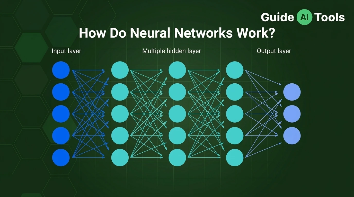
Strip away the science fiction tropes, and a neural network is not an artificial brain. It is a massive web of basic arithmetic operations multiplying inputs by adjustable knobs called weights.
Understanding how those knobs tune themselves automatically reveals how modern AI solves tasks that once baffled traditional software.
In my testing with neural network architectures, I’ve noticed that most people get overwhelmed by multivariable calculus. But the underlying mechanics are surprisingly straightforward once you break them down.
How Do Neural Networks Work? The Short Answer
Neural networks work by passing input data through layers of interconnected nodes that multiply values by adjustable weights, add biases, and apply activation functions. The system measures output error using a loss function and uses backpropagation with gradient descent to adjust weights, improving prediction accuracy over time.
Think of the entire structure as a trainable mathematical function approximator. You feed raw numbers into the input side, and the network processes those numbers through hidden layers to produce a final prediction score.
To understand how these node layers fit into broader intelligent systems, read our foundational guide on how does ai work for clear architectural context.
Every node connection acts like an adjustable valve that controls signal flow. When the output score misses the target, the network calculates its error margin and adjusts every internal valve backward.
If you want to explore the basic definitions of artificial nodes before diving deeper, check out our companion breakdown on what is a neural network to see core structural concepts.
Neural networks learn by continually refining internal numerical weights until their outputs align with real-world target data.
The Anatomy of an Artificial Neuron
The basic building block of every neural network is the artificial neuron, often called a node or perceptron.
A single node cannot do much on its own. However, when you stack thousands of them into connected layers, complex decision boundaries begin to form.
Each individual node executes five fundamental mathematical operations during every pass.
- Inputs serve as raw incoming feature values from your dataset or prior layers.
- Weights represent the relative strength or importance of each incoming connection.
- Bias acts as an adjustable offset value that shifts the activation threshold.
- Weighted sum combines all inputs multiplied by weights plus the bias value ($z = \sum (w \cdot x) + b$).
- Activation function converts the weighted sum into a non-linear output signal.
Higher positive weights amplify incoming signals, while negative weights suppress them.
Adjusting bias values gives nodes the flexibility to trigger output activations even when incoming feature values are close to zero.
The Four Step Training Pipeline
Training a neural network is an iterative loop that repeats millions of times across training epochs.
The pipeline moves through four distinct stages during every learning cycle.
- Input Data Ingestion: Loading raw features into the input layer nodes.
- Forward Propagation: Calculating weighted sums and passing signal values forward through hidden layers to produce an output prediction.
- Loss Calculation: Comparing the generated prediction against the ground-truth target value using a loss function.
- Backpropagation and Weight Update: Distributing the error backward across layers using gradient descent to adjust every weight and bias.
First, raw features enter the network at the input layer. The network makes no modifications at this entry stage; it simply passes raw values forward to the first hidden layer.
Second, signal values flow forward through every hidden layer. Nodes multiply inputs by weights, add biases, and apply non-linear transformations step by step.
Third, the final output layer generates a prediction score. The network compares this prediction to the actual target label to measure exact mathematical error.
Fourth, the training algorithm works backward from the output layer to the input layer. It calculates how much each weight contributed to the final error and updates those weights to reduce mistakes on the next pass.
Step-by-Step Arithmetic: A Single Neuron Calculation
Understanding the math becomes much easier when you work through concrete numbers instead of abstract formulas.
Let us walk through a single neuron pass using simple arithmetic.
Imagine a node receiving two input features: Input 1 is set to 2.0, and Input 2 is set to 3.0.
The connection for Input 1 has a weight of 0.5, while the connection for Input 2 has a weight of 1.5. The node carries a bias value of 0.1.
To calculate the weighted sum, multiply each input by its weight: 2.0 times 0.5 equals 1.0, and 3.0 times 1.5 equals 4.5.
Add those scaled values together along with the bias: 1.0 plus 4.5 plus 0.1 equals a total weighted sum of 5.6.
Next, pass that weighted sum of 5.6 through a Rectified Linear Unit activation function. Since ReLU simply outputs zero for negative numbers and passes positive numbers through unchanged, the final output stays 5.6.
Now assume our ground-truth target value for this sample is 8.0.
The network subtracts its output from the target: 8.0 minus 5.6 leaves a positive error margin of 2.4.
| Step | Operation | Mathematical Formula | Numerical Calculation | Output Value |
| 1 | Input Scaling | $w_1 \cdot x_1, w_2 \cdot x_2$ | $0.5 \cdot 2.0, 1.5 \cdot 3.0$ | $1.0, 4.5$ |
| 2 | Summation & Bias | $\sum (w \cdot x) + b$ | $1.0 + 4.5 + 0.1$ | $5.6$ |
| 3 | Activation Function | $\text{ReLU}(z)$ | $\max(0, 5.6)$ | $5.6$ |
| 4 | Error Comparison | $\text{Target} – \text{Output}$ | $8.0 – 5.6$ | $+2.4$ Error |
Every node pass reduces to basic multiplication and addition before activation functions reshape the output.
Why Activation Functions Drive Non-Linear Intelligence
Without activation functions, even a network with a hundred hidden layers collapses into a basic linear equation.
Linear operations can only draw straight decision lines through data points. Real-world problems like speech recognition, image classification, and natural language processing are deeply non-linear.
Activation functions introduce non-linear curves, allowing networks to bend decision boundaries around complex data clusters.
According to Stanford University’s Computer Science research on neural architectures, non-linear transformations give neural networks the ability to approximate any continuous mathematical function.
The Rectified Linear Unit, known as ReLU, is the most common activation function for hidden layers. It turns all negative values into zero and keeps positive values intact.
The Sigmoid function squashes any input value into a narrow range between 0 and 1. This makes it useful for binary classification tasks where you need a probability output.
The Softmax function handles multi-class classification problems. It converts an array of raw numerical scores into a normalized probability distribution where all outputs add up to 1.0.
If you want to see how these mathematical functions sit within broader machine learning frameworks, review our guide on what is machine learning to explore underlying model families.
Backpropagation and Gradient Descent: How Networks Learn
Generating predictions is only half the battle. A network only becomes useful when it learns how to fix its own mistakes.
Backpropagation is the mathematical engine behind neural network learning. It uses the calculus chain rule to calculate partial derivatives, measuring how much every individual weight contributed to the overall loss score.
Loss functions measure the total prediction error across your dataset. Mean Squared Error handles numerical regression tasks, while Cross-Entropy Loss evaluates classification predictions.
Once the loss function calculates total error, gradient descent steps in to optimize weight values.
Imagine standing on a foggy mountain peak in heavy rain, trying to reach the lowest valley floor without being able to see more than a few feet ahead.
You feel the slope of the ground under your boots and take a small step downward in the steepest direction.
Gradient descent does the exact same thing mathematically. It evaluates the slope of the loss curve and adjusts weights in the direction that decreases total error.
The learning rate determines how large that step is.
If your learning rate is too high, the model takes massive leaps, bouncing back and forth across the valley without reaching the bottom. If it is too low, training takes forever because steps are micro-millimetric.
| Learning Stage | Purpose | Primary Operation | Key Variable Adjusted |
| Forward Pass | Generate prediction score | Matrix multiplication & activation | None (computes outputs) |
| Loss Evaluation | Measure prediction error | Compare output to target label | Loss score ($L$) |
| Backpropagation | Assign error responsibility | Chain rule partial derivatives | Gradients ($\frac{\partial L}{\partial w}$) |
| Optimizer Update | Reduce overall error | Step in opposite direction of gradient | Weights ($w$) and Biases ($b$) |
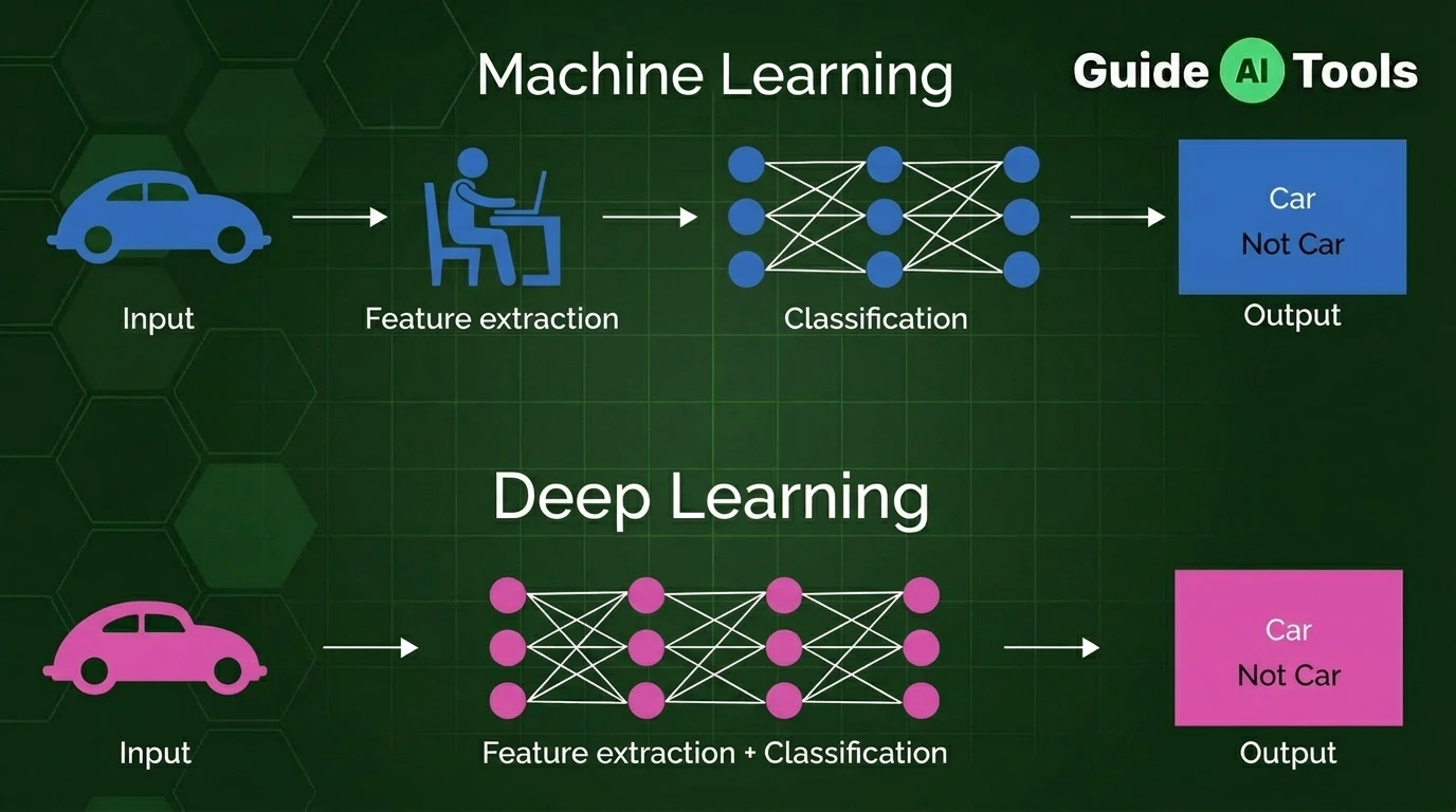
To examine how multi-layer backpropagation differs from traditional algorithms, read our breakdown on machine learning vs deep learning for a complete comparison.
For a deeper look at stacked neural layer architectures, explore our guide on what is deep learning on GuideAITools.
Backpropagation calculates exact error responsibility for every weight across the entire network hierarchy.
How Hardware Executes Neural Network Calculations
Calculating node outputs one by one on a central processing unit is far too slow for deep networks.
Modern architectures convert millions of individual node calculations into giant matrix operations.
Instead of processing one input vector at a time, hidden layers group data into matrices and run matrix dot products simultaneously.
This mathematical structure matches the physical architecture of graphics processing units (GPUs) and tensor processing units (TPUs).
Standard CPUs contain a few powerful processing cores designed for sequential tasks. GPUs contain thousands of smaller, simpler cores designed specifically for parallel matrix arithmetic.
A GPU can execute thousands of matrix multiplications concurrently. This parallel hardware execution speeds up neural network training by more than a hundred times compared to traditional CPUs.
If you want to see how this hardware scale powers modern creative tools, explore our article on what is generative ai to see foundation models in action.
FAQs
How do neural networks work step by step?
Neural networks process input features through connected node layers by multiplying values by weights, adding biases, and applying non-linear activation functions. The output error is measured by a loss function and corrected backward using backpropagation and gradient descent.
What are weights and biases in a neural network?
Weights are adjustable numerical multipliers that determine the strength of connection between nodes, while biases are offset values that allow nodes to shift their activation threshold.
What is the difference between forward propagation and backpropagation?
Forward propagation passes input data forward through layers to compute a prediction score, while backpropagation passes error calculations backward to update weights and biases.
Why do neural networks need activation functions?
Neural networks need activation functions to introduce non-linear decision boundaries, preventing multi-layer networks from collapsing into basic linear regression equations.
How does a neural network learn from its errors?
A neural network learns from errors by calculating output loss, determining partial derivatives using the chain rule, and adjusting weight parameters in the direction that lowers error.
What is gradient descent in simple terms?
Gradient descent is an optimization method that measures the slope of the error curve and takes step-by-step adjustments to find the lowest point of total prediction error.
How do GPUs make neural networks run faster?
GPUs speed up neural networks because their parallel processing cores execute thousands of matrix multiplication operations simultaneously instead of processing them sequentially.
Are artificial neural networks identical to the human brain?
No, artificial neural networks are simplified mathematical function approximators inspired by biological neurons, but they lack biological complexity, consciousness, and organic plasticity.
Conclusion
Understanding the internal mechanics of neural networks gives you a clear technical framework for evaluating modern artificial intelligence tools and deployment architectures.
When you know how weights, activation functions, and backpropagation operate under the hood, selecting the right model framework or API provider becomes much simpler.
Explore our full directory at GuideAITools to compare the top machine learning libraries, developer toolkits, and commercial AI platforms available today. Compare feature sets, review developer documentation, and pick the optimal tech stack for your next software project.

Related Blog Posts